Excel

WHAT IS THE USE OF VLOOKUP AND HOW DO WE USE IT?
The function VLOOKUP in Excel is used to look up information in a table and extract the corresponding data.
Syntax: VLOOKUP (value, table, col_index, [range_lookup])
value – Indicates the data that you are looking for in the first column of a table. (This should always be to the left of the column from where you want to retrieve the corresponding value).
table – refers to the set of data (table) from which you have to retrieve the above value.
col_index – Refers to the column in the table from where you are to retrieve the value.
range_lookup – FALSE = exact match [optional] TRUE = approximate match (default).
Shown below is an example of the VLOOKUP function:

HOW IS VLOOKUP DIFFERENT FROM THE LOOKUP FUNCTION?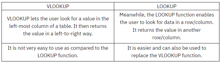

HOW DOES THE IF() FUNCTION IN EXCEL WORK?
In Excel, the IF() function performs a logical test. It returns a value if the test evaluates to true and another value if the test result is false. It returns the value depending on whether the condition is valid for the entire selected range.
Let’s look at the below example:

As seen above, the IF function returns “Record is Valid” if age is greater than 20, and the salary should be greater than $40000. Else, it will return “Record is Invalid”. Here the final answer will be “Record is Valid” as the entire selected range qualifies both the conditions.

HOW DO YOU PERFORM A HORIZONTAL LOOKUP IN EXCEL?
To perform a horizontal lookup, you will have to make use of the HLOOKUP function.
SYNTAX:
HLOOKUP(lookup_value, table_array, row_index_num, [range_lookup])
here,
lookup_value gives the value to be looked out for
table_index is the range from where the data is to be taken
row_index_num specifies the row from which you want to fetch the value
range_lookup is a logical value i.e TRUE or FALSE (TRUE will find the closest match; FALSE checks for exact match)
EXAMPLE:

WHAT ARE THE DIFFERENT TYPES OF ERRORS YOU CAN ENCOUNTER IN EXCEL?
When working with Excel, you can encounter the following six types of errors:
#N/A Error: This is called the ‘Value Not Available’ error. You will see this when you use a lookup formula and it can’t find the value (hence Not Available).
#DIV/0! Error: You’re likely to see this error when a number is divided by 0. This is called the division error.
#VALUE! Error: The value error occurs when you use an incorrect data type in a formula.
#REF! ERROR: This is called the reference error and you will see this when the reference in the formula is no longer valid. This could be the case when the formula refers to a cell reference and that cell reference does not exist (happens when you delete a row/column or worksheet that was referred in the formula).
#NAMEERROR: This error is likely to a result of a misspelled function.
#NUM ERROR: Number error can occur if you try and calculate a very large value in Excel. For example, =194^643 will return a number error.

WHAT ARE THE KNOWN LIMITATIONS OF THE VLOOKUP FUNCTION?
The VLOOKUP function is mighty useful, but it also has a few limitations:
It cannot be used when the lookup value is on the right. For VLOOKUP to work, the lookup value should always be in the left-most column. Now this limitation can be overcome by using it with other formulas, it tends to make formulas complex.
VLOOKUP would give a wrong result if you add/delete a new column in your data (as the column number value now refers to the wrong column). You can make the column number dynamic, but if you planning to combine two or more functions, why not use INDEX/MATCH in the first place.
When used on large data sets, it can make your workbook slow.

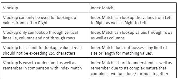
WHAT IS THE DIFFERENCE BETWEEN VLOOKUP AND INDEX MATCH FUNCTION?

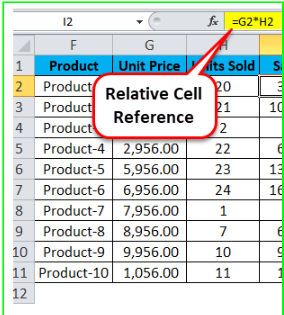
WHAT IS RELATIVE CELL REFERENCING IN EXCEL?
Relative cell referencing is used when dealing with formulas in Excel. If you write a sum formula to add the values of a set of cells (e.g A4 to A8) together, it will look like this: =SUM(A4:A8). If you use relative cell references, then when you copy this formula to a different section of the spreadsheet, the cells will change relative to where the formula has been pasted. For example, if you copy the formula across one column, the formula will become =SUM(B4:B8).

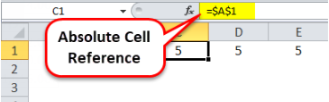
WHAT IS ABSOLUTE CELL REFERENCING ?
Absolute cell referencing is the exact opposite of relative cell referencing. By marking the row number and column letter with a $ symbol, you can make a cell reference fixed (or “absolute”). This means that when you copy and paste it to another cell or use AutoFill, the cell references will not change. The formula =SUM(A4:A8) will stay as =SUM(A4:A8) no matter where you put it.

WHAT IS THE DIFFERENCE BETWEEN COUNT , COUNTA, COUNTBLANK AND COUNTIF IN EXCEL?
COUNT: This function counts how many cells within a specified range contain numerical data. It will ignore (not count) any cells that are blank or contain text or symbols only.
COUNTA: This function counts how many cells within a specified range contain data of any type. It will count all cells that are not blank.
COUNTBLANK: This function will count the number of blank cells within the designated range.
COUNTIF: This function will count only the cells whose value meets a certain condition specified by the user.

WHAT IS A PIVOT TABLE?
A pivot table is a tool in data summation that is common in many business software. It is utilized to collect the summary of a specific data set in a compressed technique. It is a very useful tool in consolidating a large quantity of data that is contained in Microsoft Excel. They let the user make a faster organization and drawing of conclusions from data being collected. Pivot table consists of columns, rows, pages, and data fields. These can be moved around and it assists in expanding, isolating, summarizing, and grouping the specific data. And all of these can be accomplished in real time.

ADVANTAGES AND DISADVANTAGES OF PIVOT TABLE?
Advatages of Pivot Table are:
Pivot tables allow you to see how your data works
Works well with SQL exports
Large amounts of data can be segmented
Creating instant data is possible
Disadvantages of Pivot Table are:
Mastering pivot tables takes time
Can be time-consuming to use
There are no automatic updates
Older computers might not be able to handle large data sets

WHAT IS DATA VALIDATION?
Data Validation restricts the type of values that a user can enter into a particular cell or a range of cells.
In the Data tab, select the ‘Data Validation’ option present under Data Tools.

Select the kind of data validation you want to apply.

HOW DO YOU HYPERLINK IN EXCEL?
To create a link in Excel, select the element you wish to use as the anchor (this can be a cell or an object like a picture). You can then either select Link from the Insert tab, right-click and select Link on the menu, or press Ctrl+K.  This will bring up a variety of options that will allow you to indicate what kind of content you would like to link to, such as a file, a web page, a specific location, or an email address.

WHAT IS SOLVER?
Solver in Excel is an add-in that allows you to get an optimum solution when there are many variables and constraints. You can consider it to be an advanced version of Goal Seek.
With Solver, you can specify what the constraints are and the objective that you need to achieve. It does the calculation in the back-end to give you a possible solution.

WHAT ARE MACROS IN EXCEL? CREATE A MACRO TO AUTOMATE A TASK.
Macro is a program that resides within the Excel file. The use of it is to automate repetitive tasks that you would like to perform in Excel.
To record a macro, you can either go to the Developer tab and click on Record Macro or access it from the View tab.

HOW WOULD YOU HIGHLIGHT CELLS WITH DUPLICATE VALUES IN IT?
You can do this easily using conditional formatting. Here are the steps:
a) Select the data in which you want to highlight duplicate cells.
b) Go to the Home tab and click on the Conditional Formatting option.
c) Go to Highlight Cell Rules and click on ‘Duplicate Values’ option.

HOW CAN WE COMBINE TEXT STRINGS FROM MULTIPLE CELLS IN A SINGLE CELL?
You can use the CONCATENATE() function to combine text strings from multiple cells into a single cell.
The “&” operator can also be used to combine cell values.

HOW TO CREATE A DROP-DOWN LIST IN EXCEL?
This can be accomplished by selecting the ‘Data Validation’ option from the Data tab.

WHAT IS THE PURPOSE OF NESTED IF?
Because we have several conditions to satisfy, we can use the IF function seven times, which is known as the Nested IF function.

HOW DO WE USE THE SUMIF() FUNCTION IN EXCEL?
SUMIF() adds the cell values specified by a given condition or criteria.